According to Nernst distribution law, a solute can distribute itself between two immiscible solvents in contact in such a way that the ratio of its concentration in these solvents at equilibrium conditions is constant at a given temperature. When a solute distributes itself between two immiscible solvents, there is a definite relationship between the solute concentration in the two phases at equilibrium. To explain this relation, Nernst gave this law in 1891, known as the distribution law.
Nernst distribution law
This law can be stated as ” At constant temperature, when two solutions of a solute in two immiscible solvents are in contact with each other, then solute distributes itself to keep a fixed ratio of concentration in the two immiscible solvents at equilibrium.
If a solute S distributes itself between two immiscible solvents of phase 1( aqueous solvent) and phase 2(organic solvent) at equilibrium, the ratio of the concentration of solute in phases 1 and 2 remains the same at a constant temperature. If [S1] is the concentration of solute in phase 1 and [S2] is the concentration of solute in phase 2, then at equilibrium, distribution coefficient Kd is expressed as:

Nernst distribution law holds true under the following conditions:
- The temperature should remain constant. Otherwise, the value of the distribution coefficient changes by changing the temperature.
- The solute should not undergo association or dissociation i.e it should be present in the same molecular form in both solvents.
- Solute should not react with either solvent.
- The concentration of solute should be low.
Nernst distribution law derivation
Let a solute is soluble in solvent A and solvent B such that solvent A and solvent B are immiscible with each other.
Let, µ(A)= Chemical potential of the solute in solvent A.
µ(B)= Chemical potential of the solute in solvent B.
µo(A)= Standard chemical potential of the solute in solvent A.
µo(B)=Standard chemical potential of the solute in solvent B.
aA= Activity of the solute in solvent A.
aB=activity of the solute in solvent B.
The chemical potential of solute is solvent A can be given as
µ(A)=µo(A) + RTlnaA
Similarly, For in solvent B,
µ(B)=µo(B) + RTlnaB
Where R is the universal gas constant and T is the temperature in Kelvin.
When the solution of the solute in solvent A is mixed with a solution of the solute in solvent B then, at equilibrium the chemical potential µ(A) and µ(B) become equal.
At equilibrium, µ(A)=µ(B)
µo(A) + RTlnaA=µo(B) + RTlnaB
µo(A)–µo(B)=RTlnaB–RTlnaA
µo(A)–µo(B)=RT In (aA/aB)
µo(A)–µo(B)/RT=In (aA/aB)
At a particular temperature, µo(A), µo(B), and R are constant.
In (aA/aB)= Constant.
Taking antilog on both sides,
aA/aB= K …………………….(i)
This equation is the mathematical expression of the Nernst distribution law.
For dilute solution, equation(i) can be modified as,
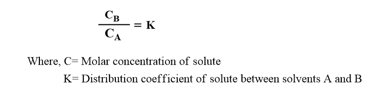
Application of Nernst distribution law
- It can be used to determine the solubility of a substance.
- It is applicable in solvent extraction.
- This is useful in Parke’s process of desilverization of lead.
- This is used in the determination of the equilibrium constant of a chemical equilibrium involving the formation of complex ions.
- With the help of this law, we can determine the value of the molecular complexity of the solute.
Limitations of Nernst distribution law
- This law does not hold true when solutes undergo ionization or dissociation.
- If solute combines with one or both of the solvents, then this law does not hold true.
- If the mutual solubility of two solvents is affected due to the presence of solute, the law does not hold true.
- The law holds true for only ideal solutions only.
References:
- S. M. Khopkar, Basic Concepts of Analytical Chemistry, (3rd Edition), New Age International Pvt. Ltd., New Delhi, India (2008).